Unraveling the Database Optimizer

Here at Outschool, our primary transactional data store is a relational Postgres database. As such, it is not uncommon that we encounter optimization problems involving database queries.

At a recent company lunch-n-learn, we unpacked a few basic concepts to help dismantle the bogey man that is the database optimizer. To some engineers, the optimizer is a mysterious black box that often has to be cajoled through sleight of hand to do the right thing. However, given a set of inputs, the optimizer is actually predictably deterministic. An understanding of how the optimizer makes decisions empowers us to make better decisions ourselves while fine-tuning query performance.

In this blog post, we’ll briefly review a few of the concepts presented at the lunch-n-learn.

Gut Feel vs. the Optimizer

Recently, our team launched a popular feature that allows learners to self-discover classes. Learners can now search for classes and save them to their Favorites list. Imagine that we wanted to query for a list of classes saved by learners. Our query might look something like this:

SELECT user_favorites.*
FROM
  user_favorites
  JOIN users
    ON user_favorites.user_id = users.id
WHERE
  users.is_learner = TRUE;

Now, imagine that I rewrote the query by moving the filter into the JOIN condition.

SELECT user_favorites.*
FROM
  user_favorites
  JOIN users
    ON user_favorites.user_id = users.id
    AND users.is_learner = TRUE;

Which query do you think would perform better? When I posed this question at the lunch-n-learn, the consensus was that the second query should perform better than the first, because it was restricting the users table before joining it with user_favorites. Sounds logical; and yet surprisingly, both queries actually generate the exact same query plan. Here’s what that plan looks like:

Gather  (cost=967.85..3835.44 rows=6922 width=3240)
  Workers Planned: 2
  ->  Parallel Hash Join  (cost=967.85..2069.24 rows=2376 width=3240)
        Hash Cond: (user_favorites.user_id = users.id)
        ->  Parallel Seq Scan on user_favorites  (cost=0.00..781.54 rows=5654 width=487)
        ->  Parallel Hash  (cost=628.99..628.99 rows=659 width=253)
              ->  Parallel Seq Scan on users  (cost=0.00..628.99 rows=659 width=253)
                    Filter: is_learner

* Cost and row counts do not represent real numbers

Query plans should be read from the bottom up. Notice that in this plan, the very first thing that happens is that the is_learner filter is applied to the users table! Even though the first query we wrote filtered the data after the join, the database was smart enough to realize that it would be more optimal to constrict the data first. How did the optimizer arrive at this conclusion?

Decisions, Decisions, Decisions

Given a query, the first thing the database does is to lay out all possible ways in which the data being requested could be retrieved. There are three main variables that determine the different permutations of execution strategies available for any given query - scan strategies, join strategies and join order.

Scan Strategies

Simplistically, the database engine has a couple of options when it comes to retrieving data from the table file. One of those is the sequential scan - where data is directly pulled from the table file sequentially. A second option is the index scan - where the data is first filtered on the index, and filtered rows being pointed to by the index are pulled from the table file.

While you may have been taught that sequential scans are all bad, that isn’t strictly true. Consider for instance a query where you just want to pull the first 100 rows from a table without any consideration for sort order. In this instance, the one-step sequential scan to pull the top 100 rows is actually preferable to the two-step index scan. If you now decide to sort that same query on an indexed column, the index scan becomes preferable.

Join Strategies

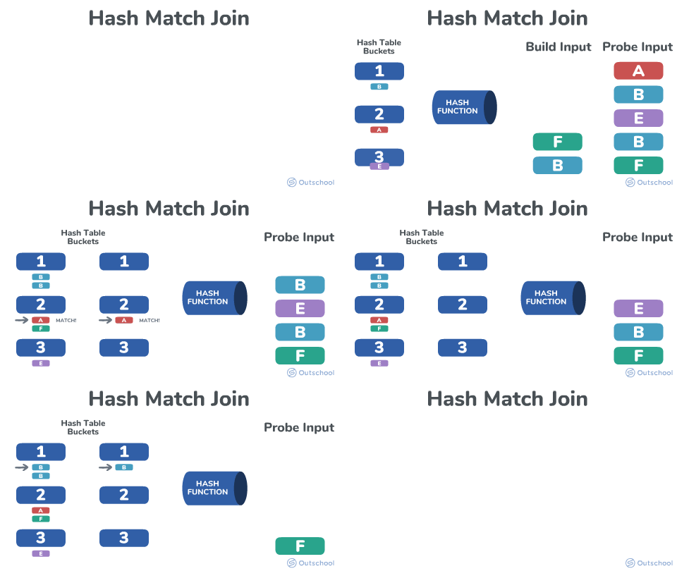
These determine how a join is performed. Options include a nested loop (the first dataset is scanned in an outer loop; the second dataset is scanned for matches in an inner loop); a merge join (both datasets are first sorted using the join key and then sequentially scanned in parallel for matches); and a hash join (involves a build phase where a hash is built from the first dataset and a probe phase where each row of the second dataset is is converted to a hash and the second dataset is looped through, performing hash lookups for matches with the first dataset).

* Animation inspired by the work of Bert Wagner

Here again, one strategy isn’t necessarily better than the other. The costs are distributed differently in each case - whether it is the inner loop in the first strategy, the sorting cost of the merge join or the hash creation/lookup costs in the hash join. Whereas nested loops might be a better option when at least one of the two datasets being joined is small, that same query might prefer a hash or merge strategy when joining two large datasets.

Estimating Costs

Given the possible permutations between scan strategies, join strategies and join order, Postgres uses a cost-based approach to determining the optimal plan for a given query. Postgres uses statistics that it maintains on each table to assign an estimated cost to each operation of a given plan. These costs drive the optimizer’s decision on which plan to use. A discrepancy between the estimated cost and actual time of a given operation is an indicator that perhaps the planner’s statistics need to be updated.

In Conclusion

Confidence in reading a query plan to understand the optimizer’s rationale is a key first step in determining how to optimize a query. It allows us to make decisions such as,

1. Does the query need to be re-written (for instance, aggregating post join vs. aggregating in a subquery prior to a join)?
2. Should we index the data differently?
3. Do the planner’s statistics need to be updated?
4. Would it be preferable to query for a raw dataset and perform data manipulation (such as sorting and aggregation) outside of the query?
5. Would a large query benefit from being broken into multiple smaller queries?
6. Should we negotiate the business requirements surrounding the query to provide the best UX?

In future, we hope to return to this topic with an analysis of specific queries we’ve optimized here at Outschool. But for now, hopefully you share our team’s confidence in being able to easily decipher what the optimizer’s trying to tell us.

For Further Reading

• Overview of PostgreSQL Internals: Planner/Optimizer
• Winand, M. The Join Operation
• Kerstiens, C. More on Postgres Performance